ml-models-exercise

Author

Cassia Roth

Published

March 25, 2024

Load the data and set the seed for reproducibility.

#Loading packages
library(tidyverse) #This includes ggplot2, tidyr, readr, dplyr, stringr, purr, forcats
library(tidymodels) #This includes recipes, rsample, parsnip, yardstick, and dials
library(here) # For file paths
library(dials) # For tuning models

#Path to summary data. Note the use of the here() package and not absolute paths
data_location <- here::here("fitting-exercise","mavoglurant.rds")

#load data
mavo_ml<- readRDS(data_location)

# Fix the random numbers by setting the seed 
# This enables the analysis to be reproducible when random numbers are used 
rngseed = 1234

More processing

I can’t figure out the meaning of the numbers for the RACE variable. Nonetheless, here, we will recode so that RACE has three levels: 1, 2, and 3.

# Define "3" as a new level if it doesn't exist
mavo_ml$RACE <- fct_expand(mavo_ml$RACE, "3")

# Combine categories 7 and 88 into category 3
mavo_ml <- mavo_ml %>%
  mutate(RACE = fct_collapse(RACE, "3" = c("7", "88")))
mavo_ml

# A tibble: 120 × 7
       Y  DOSE   AGE SEX   RACE     WT    HT
   <dbl> <dbl> <dbl> <fct> <fct> <dbl> <dbl>
 1 2691.    25    42 1     2      94.3  1.77
 2 2639.    25    24 1     2      80.4  1.76
 3 2150.    25    31 1     1      71.8  1.81
 4 1789.    25    46 2     1      77.4  1.65
 5 3126.    25    41 2     2      64.3  1.56
 6 2337.    25    27 1     2      74.1  1.83
 7 3007.    25    23 1     1      87.9  1.85
 8 2796.    25    20 1     3      61.9  1.73
 9 3866.    25    23 1     2      65.3  1.65
10 1762.    25    28 1     1     104.   1.84
# ℹ 110 more rows

Pairwise correlations

We will now make pairwise correlations for the continuous variables, removing any variables that show very strong correlations.

# Check continuous variables (Y, DOSE, AGE, WT, HT). Even though DOSE could be considered categorical...
str(mavo_ml)

tibble [120 × 7] (S3: tbl_df/tbl/data.frame)
 $ Y   : num [1:120] 2691 2639 2150 1789 3126 ...
 $ DOSE: num [1:120] 25 25 25 25 25 25 25 25 25 25 ...
 $ AGE : num [1:120] 42 24 31 46 41 27 23 20 23 28 ...
 $ SEX : Factor w/ 2 levels "1","2": 1 1 1 2 2 1 1 1 1 1 ...
 $ RACE: Factor w/ 3 levels "1","2","3": 2 2 1 1 2 2 1 3 2 1 ...
 $ WT  : num [1:120] 94.3 80.4 71.8 77.4 64.3 ...
 $ HT  : num [1:120] 1.77 1.76 1.81 1.65 1.56 ...

# Select the continuous variables
continuous_vars <- select_if(mavo_ml, is.numeric)

# Calculate the correlation matrix
correlation_matrix <- cor(continuous_vars)

# Convert correlation matrix to a data frame
mavo_cor <- as.data.frame(correlation_matrix)

# Add row names as a column
mavo_cor$vars <- rownames(mavo_cor)

# Reshape the data to long format
correlation_long <- pivot_longer(mavo_cor, cols = -vars, names_to = "Variable_1", values_to = "Correlation")

# Create a ggplot for the correlation plot
mavo_plot_cor <- ggplot(data = correlation_long, aes(x = vars, y = Variable_1, fill = Correlation)) +
  geom_tile(color = "white") +
  scale_fill_gradient2(low = "blue", high = "red", mid = "white", 
                       midpoint = 0, limit = c(-1,1), space = "Lab",
                       name="Correlation") +
  theme_minimal() +
  theme(axis.text.x = element_text(angle = 45, vjust = 1, size = 10, hjust = 1)) +
  labs(x = "Variables", y = "Variables") +
  coord_fixed()
mavo_plot_cor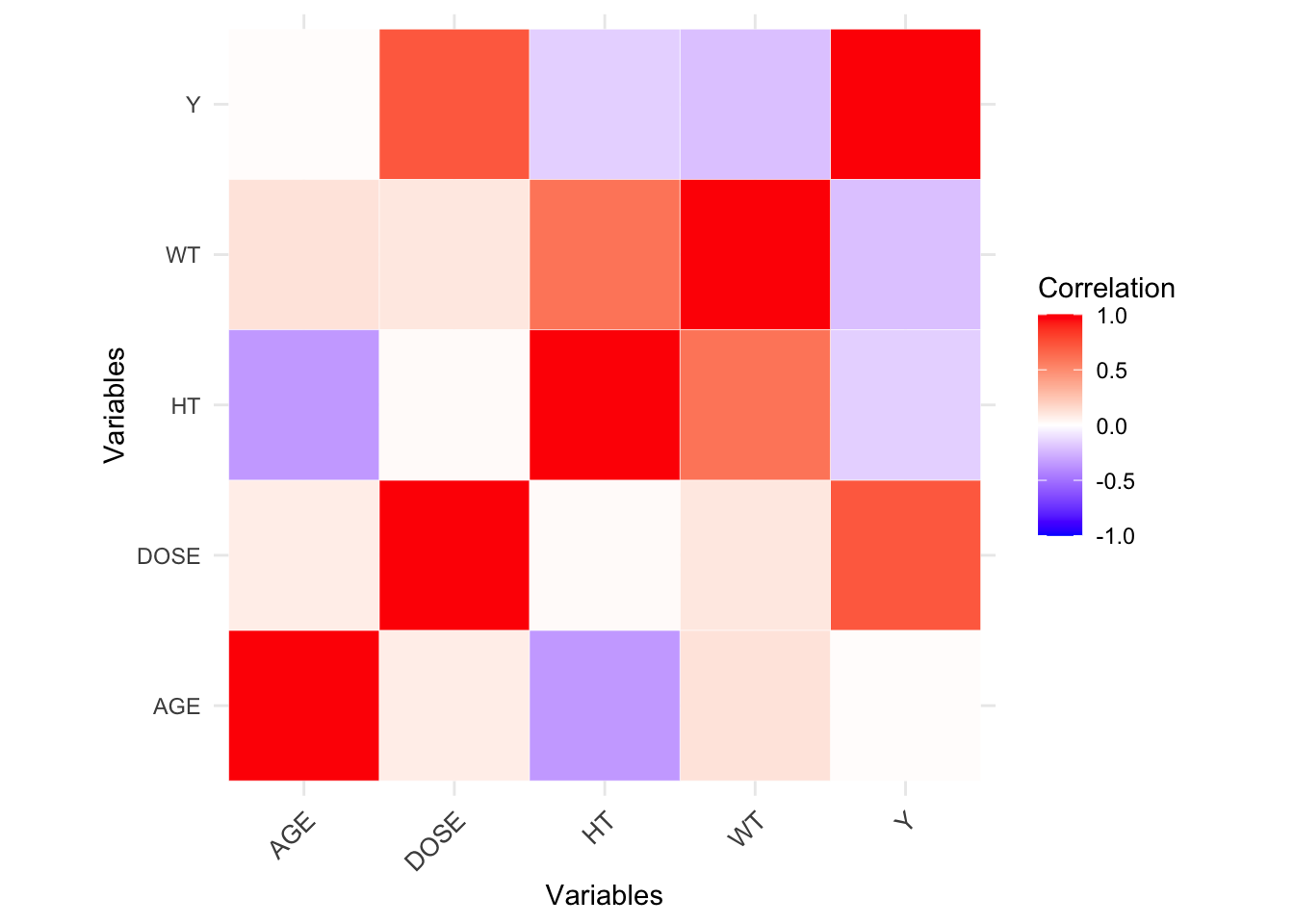

# Save figure
figure_file <- here("ml-models-exercise", "correlation_plot.png")
ggsave(filename = figure_file, plot=mavo_plot_cor, bg="white")

Some variables appear to be strongly correlated, but nothing is excessive (|>0.9|).

Feature Engineering

Don’t worry: feature engineering is just a “fancy” phrase for creating new variables. First we will create a new variable called BMI. Our measurements for height and weight are in the metric system (centimeters and kilograms, accordingly). According to the CDC the formula for BMI is: \([weight (kg) / [height (m)]^2\).

# Create a new variable called BMI
mavo_ml <- mavo_ml %>%
  mutate(BMI = (WT / (HT^2)))
mavo_ml

# A tibble: 120 × 8
       Y  DOSE   AGE SEX   RACE     WT    HT   BMI
   <dbl> <dbl> <dbl> <fct> <fct> <dbl> <dbl> <dbl>
 1 2691.    25    42 1     2      94.3  1.77  30.1
 2 2639.    25    24 1     2      80.4  1.76  26.0
 3 2150.    25    31 1     1      71.8  1.81  21.9
 4 1789.    25    46 2     1      77.4  1.65  28.4
 5 3126.    25    41 2     2      64.3  1.56  26.4
 6 2337.    25    27 1     2      74.1  1.83  22.1
 7 3007.    25    23 1     1      87.9  1.85  25.7
 8 2796.    25    20 1     3      61.9  1.73  20.7
 9 3866.    25    23 1     2      65.3  1.65  24.0
10 1762.    25    28 1     1     104.   1.84  30.6
# ℹ 110 more rows

Model Building

Now we will explore 3 different models: 1) a linear model with all predictors; 2) a LASSO regression; 3) a random forest (RF).

First, let’s make sure we have the glmnet and ranger packages installed and loaded.

# Install and load needed packages
#install.packages("glmnet")
#install.packages("ranger")
library(glmnet)
library(ranger)

# ChatGPT, GitHub CoPilot and looking at Kevin Kosewick's code helped me to write this code.
# Set seed for reproducibility
set.seed(rngseed)

# Define outcome and predictors
outcome <- "Y"
predictors <- setdiff(names(mavo_ml), outcome)

# Create recipe for linear and LASSO models (creating dummy variables and standardizing continuous variables)
mavo_recipe_lmlasso <- recipe(Y ~ ., data = mavo_ml) %>%
  step_dummy(all_nominal(), -all_outcomes()) %>%
  step_normalize(all_predictors())

# Create recipe for random forest model (no need to create dummy variables or standardize continuous)
mavo_recipe_rf <- recipe(Y ~ ., data = mavo_ml)

# Define models
# Linear model
mavo_lm <- linear_reg() %>%
  set_engine("lm") %>%
  set_mode("regression")

# LASSO model
mavo_LASSO <- linear_reg(penalty = 0.1, mixture = 1) %>%
  set_engine("glmnet") %>%
  set_mode("regression")

# Random forest model
mavo_rf <- rand_forest() %>%
  set_engine("ranger", seed = rngseed) %>%
  set_mode("regression")

# Create workflows
# Linear workflow
linear_workflow <- workflow() %>%
  add_recipe(mavo_recipe_lmlasso) %>%
  add_model(mavo_lm)

# LASSO workflow
LASSO_workflow <- workflow() %>%
  add_recipe(mavo_recipe_lmlasso) %>%
  add_model(mavo_LASSO)

# Random forest workflow
rf_workflow <- workflow() %>%
  add_recipe(mavo_recipe_rf) %>%
  add_model(mavo_rf)

# Fit models
#Linear
linear_fit <- linear_workflow %>%
fit(data = mavo_ml)

# LASSO
LASSO_fit <- LASSO_workflow %>%
  fit(data = mavo_ml)

# Random forest
rf_fit <- rf_workflow %>%
  fit(data = mavo_ml)

# Tidy all results linear and LASSO
linear_fit_results <- tidy(linear_fit, fmt = "decimal")
linear_fit_results

# A tibble: 9 × 5
  term        estimate std.error statistic  p.value
  <chr>          <dbl>     <dbl>     <dbl>    <dbl>
1 (Intercept)   2445.       54.3    45.1   3.45e-73
2 DOSE           701.       56.1    12.5   6.22e-23
3 AGE             40.7      67.1     0.607 5.45e- 1
4 WT            1822.      745.      2.45  1.60e- 2
5 HT           -1440.      490.     -2.94  4.00e- 3
6 BMI          -1715.      601.     -2.85  5.20e- 3
7 SEX_X2        -148.       71.7    -2.07  4.06e- 2
8 RACE_X2         72.7      57.2     1.27  2.07e- 1
9 RACE_X3        -71.5      59.6    -1.20  2.33e- 1

LASSO_fit_results <- tidy(LASSO_fit)
LASSO_fit_results

# A tibble: 9 × 3
  term        estimate penalty
  <chr>          <dbl>   <dbl>
1 (Intercept)   2445.      0.1
2 DOSE           702.      0.1
3 AGE             39.7     0.1
4 WT            1713.      0.1
5 HT           -1369.      0.1
6 BMI          -1627.      0.1
7 SEX_X2        -147.      0.1
8 RACE_X2         72.5     0.1
9 RACE_X3        -69.7     0.1

# Extract info from random forest
rf_fit_results <- rf_fit$.workflow[[1]]$fit$fit$forest$importance %>%
  as_tibble()
rf_fit_results

# A tibble: 0 × 0

Now we will use the model to make predictions on the entire dataset, reporting the RMSE performance metric for each of the three model fits. Finally, we will make an observed versus predicted plot for each of the models.

# ChatGPT and GitHub CoPilot helped with this code.

# Make predictions
# linear model
linear_preds <- predict(linear_fit, mavo_ml) %>%
  bind_cols(mavo_ml) %>% # alternative way to augment (adding columns to dataset with observed and predicted values)
  select(Y, pred = .pred)

# LASSO model
LASSO_preds <- predict(LASSO_fit, mavo_ml) %>%
  bind_cols(mavo_ml) %>% # alternative way to augment (adding columns to dataset with observed and predicted values)
  select(Y, pred = .pred)

# Random forest model
rf_preds <- predict(rf_fit, mavo_ml) %>%
 bind_cols(mavo_ml) %>% # alternative way to augment (adding columns to dataset with observed and predicted values)
select(Y, pred = .pred)

# Get RMSE for each model
# linear model
linear_rmse <- rmse(linear_preds, truth = Y, estimate = pred)
linear_rmse

# A tibble: 1 × 3
  .metric .estimator .estimate
  <chr>   <chr>          <dbl>
1 rmse    standard        572.

# LASSO model
LASSO_rmse <- rmse(LASSO_preds, truth = Y, estimate = pred)
LASSO_rmse

# A tibble: 1 × 3
  .metric .estimator .estimate
  <chr>   <chr>          <dbl>
1 rmse    standard        572.

# Random forest model
rf_rmse <- rmse(rf_preds, truth = Y, estimate = pred)
rf_rmse

# A tibble: 1 × 3
  .metric .estimator .estimate
  <chr>   <chr>          <dbl>
1 rmse    standard        358.

# Print RMSE values
print(paste("Linear Model RMSE: ", linear_rmse[[3]]))

[1] "Linear Model RMSE:  571.595397430179"

print(paste("LASSO Model RMSE: ", LASSO_rmse[[3]]))

[1] "LASSO Model RMSE:  571.650382196397"

print(paste("Random Forest Model RMSE: ", rf_rmse[[3]]))

[1] "Random Forest Model RMSE:  358.431791306429"

# Create observed versus predicted plots
linear_preds_plot <- ggplot(linear_preds, aes(x = Y, y = pred)) +
  geom_point() +
  geom_abline(slope = 1, intercept = 0, color = "red") +
  labs(title = "Observed vs Predicted (Linear Model)", x = "Observed", y = "Predicted")

LASSO_preds_plot <- ggplot(LASSO_preds, aes(x = Y, y = pred)) +
  geom_point() +
  geom_abline(slope = 1, intercept = 0, color = "red") +
  labs(title = "Observed vs Predicted (LASSO Model)", x = "Observed", y = "Predicted")

rf_preds_plot <- ggplot(rf_preds, aes(x = Y, y = pred)) +
  geom_point() +
  geom_abline(slope = 1, intercept = 0, color = "red") +
  labs(title = "Observed vs Predicted (Random Forest Model)", x = "Observed", y = "Predicted")

# Display plots
linear_preds_plot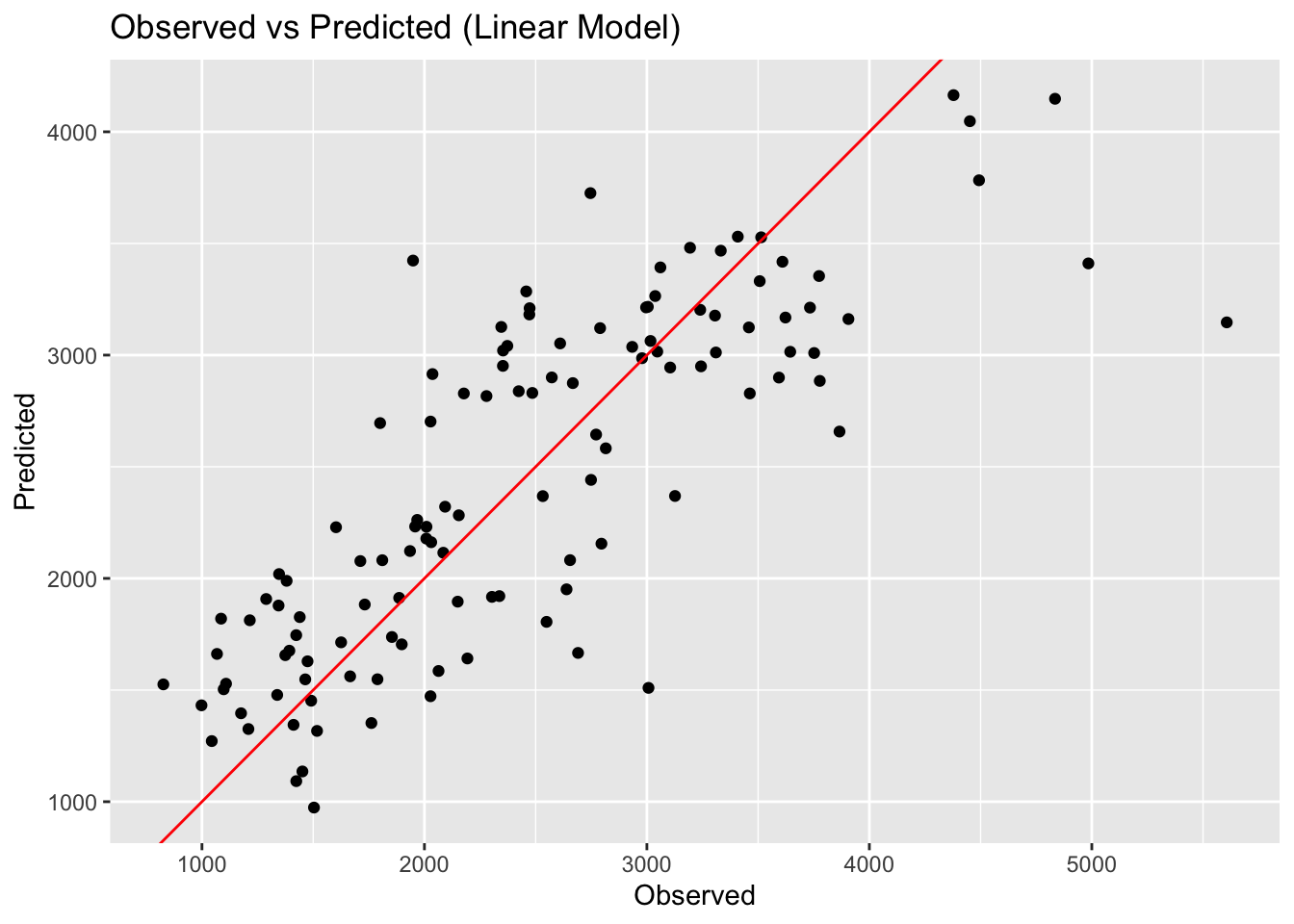

LASSO_preds_plot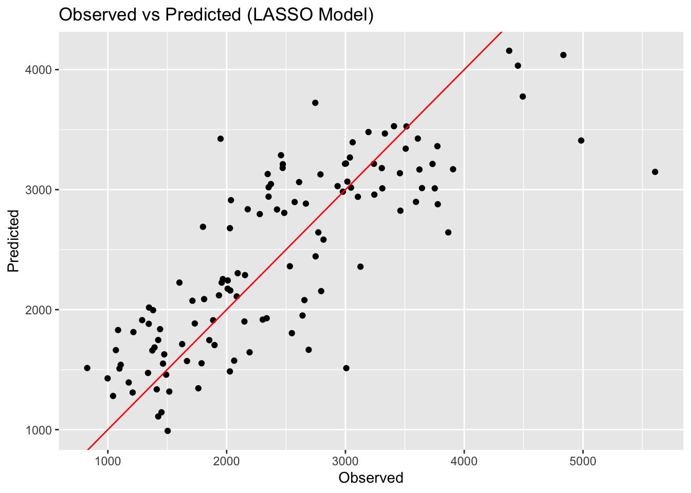

rf_preds_plot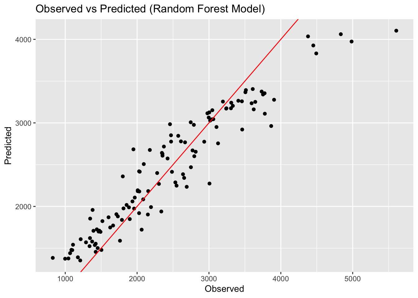

# Save plots
figure_file <- here("ml-models-exercise", "linearplot.png")
ggsave(filename = figure_file, plot=linear_preds_plot, bg="white")

figure_file <- here("ml-models-exercise", "LASSOplot.png")
ggsave(filename = figure_file, plot=LASSO_preds_plot, bg="white")

figure_file <- here("ml-models-exercise", "rfplot.png")
ggsave(filename = figure_file, plot=rf_preds_plot, bg="white")

Here we can see that the linear model and LASSO model give very similar results. LOOK BACK AT WHY. The random forest model performs best, with an RMSE of 358. The scatterplots of the observed versus predicted values reinforces this point, with the random forest model having the least amount of variation. This isn’t surprising as we know that random forest models are flexible and can capture patterns in the data well.

Tuning the models

We will now tune the LASSO and RF models to improve model performance. Unlike in a real-data situation, we will be doing this without cross-validation for educational purposes even though we know this will overfit our data. Let’s start with our LASSO model.

For the LASSO model, we will define a grid of parameters to tune over from 1E-5 to 1E2 (50 values linearly spaced on a log scale). We will use the tune_grid() function to tune the model by testing model performance for each parameter value defined in the search grid. To create an object that only contains the data and for which we can use as resamples input for tune_grid(), we will use the apparent() function. Finally, we will look at the diagnostics using autoplot().

#ChatGPT and Zane Billings helped with this code
# Set seed for reproducibility
set.seed(rngseed)

# Tune LASSO model

# Create recipe for LASSO tune model
mavo_recipe_LASSO_tune <- recipe(Y ~ ., data = mavo_ml) %>%
   step_normalize(all_numeric_predictors()) %>%
  step_dummy(all_nominal_predictors())

# Define LASSO model
mavo_LASSO_tune <- linear_reg(penalty = tune(), mixture = 1) %>%
  set_engine("glmnet") %>%
  set_mode("regression")

# Define penalty parameter with your range (used this website: https://dials.tidymodels.org/reference/penalty.html)
penalty_param <- penalty(range = c(-5, 2), trans = transform_log10())

# Define search grid for tuning
lasso_grid <- grid_regular(penalty_param, levels = 50)

# Create workflow for tuning
LASSO_tune_wf <- workflow() %>%
  add_recipe(mavo_recipe_LASSO_tune) %>%
  add_model(mavo_LASSO_tune)

# Create resamples object using apparent
apparent_resamples <- apparent(mavo_ml)

# Tune the LASSO model
LASSO_tune_results <- tune_grid(
  object = LASSO_tune_wf,
  resamples = apparent_resamples,
  grid = lasso_grid,
  metrics = metric_set(rmse)
)

autoplot(LASSO_tune_results)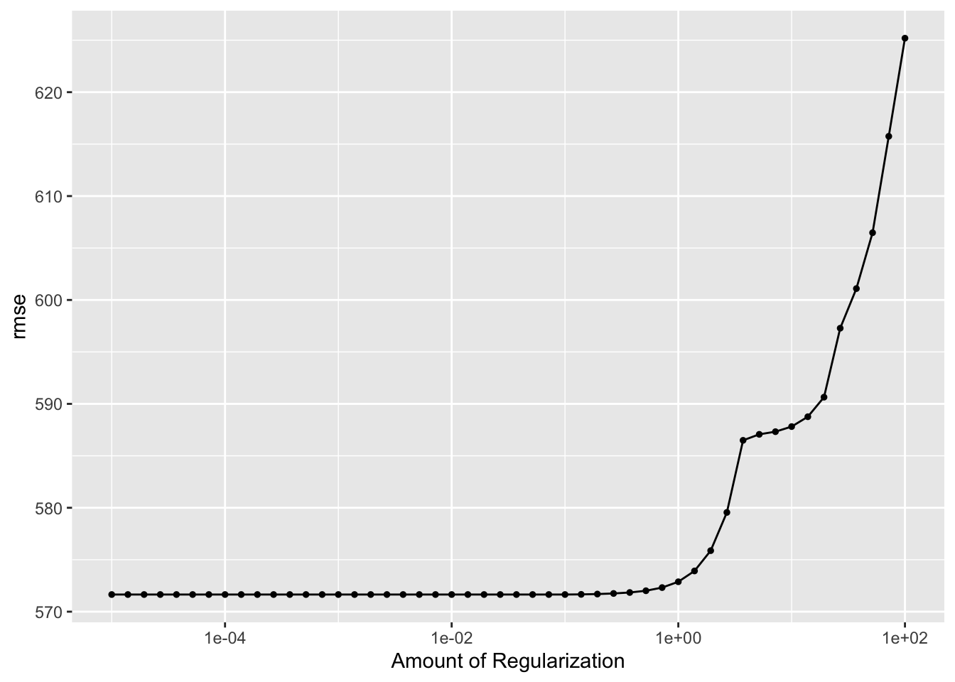

# Get RMSE from tuning results
rmse_values <- collect_metrics(LASSO_tune_results) %>%
  filter(.metric == "rmse")
rmse_values

# A tibble: 50 × 7
     penalty .metric .estimator  mean     n std_err .config              
       <dbl> <chr>   <chr>      <dbl> <int>   <dbl> <chr>                
 1 0.00001   rmse    standard    572.     1      NA Preprocessor1_Model01
 2 0.0000139 rmse    standard    572.     1      NA Preprocessor1_Model02
 3 0.0000193 rmse    standard    572.     1      NA Preprocessor1_Model03
 4 0.0000268 rmse    standard    572.     1      NA Preprocessor1_Model04
 5 0.0000373 rmse    standard    572.     1      NA Preprocessor1_Model05
 6 0.0000518 rmse    standard    572.     1      NA Preprocessor1_Model06
 7 0.0000720 rmse    standard    572.     1      NA Preprocessor1_Model07
 8 0.0001    rmse    standard    572.     1      NA Preprocessor1_Model08
 9 0.000139  rmse    standard    572.     1      NA Preprocessor1_Model09
10 0.000193  rmse    standard    572.     1      NA Preprocessor1_Model10
# ℹ 40 more rows

# Save file
figure_file <- here("ml-models-exercise", "LASSO_tune_plot.png")
ggsave(filename = figure_file, plot=autoplot(LASSO_tune_results), bg="white")

As the penalty parameter increases, the lambda in the cost function is increasing. Since it uses the absolute values of the coefficients, the sum of the coefficients is always positive. Therefore, as the lambda increases the value of the regularization term increases, which makes the RMSE larger.

Now let’s repeat this with the random forest model.

#ChatGPT and the links below helped with this code
# Set seed for reproducibility
set.seed(rngseed)

# Create new recipe for random forest tuning model
mavo_recipe_rf_tune <- recipe(Y ~ ., data = mavo_ml)

#Define model specification using ranger
rf_spec <-
  rand_forest(mode = "regression",
              mtry = tune(),
              min_n = tune(),
              trees = 300) %>% # number of trees
  set_engine("ranger", seed = rngseed)

# Create workflow for tuning
rf_tune_wf <- workflow() %>%
  add_model(rf_spec) %>%
  add_recipe(mavo_recipe_rf_tune)

# Define the parameter mtry and create a grid for tuning, Used this website: https://dials.tidymodels.org/reference/mtry.html
mtry_grid <- mtry(range = c(1, 7)) %>%
             grid_regular(levels = 7)

# Define the parameter min_n and create a grid for tuning. Used this website: https://dials.tidymodels.org/reference/trees.html
min_n_grid <- min_n(range = c(1, 21)) %>%
             grid_regular(levels = 7)

# Combine grids
param_grid <- expand_grid(mtry_grid, min_n_grid)

# Create resamples object using apparent
#apparent_resamples <- apparent(mavo_ml)

# Tune with control parameters
rf_tune_results <- rf_tune_wf %>% tune_grid(
  resamples = apparent_resamples,
  grid = param_grid,
  metrics = metric_set(rmse)
)

# Observe process
rf_tune_results %>% autoplot()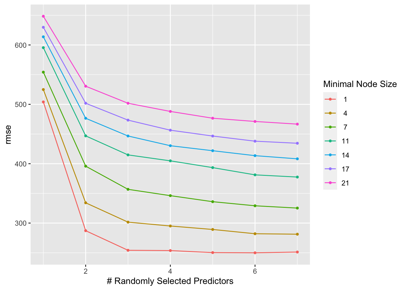

# Get RMSE from tuning results
rmse_values <- collect_metrics(rf_tune_results) %>%
  filter(.metric == "rmse")
rmse_values

# A tibble: 49 × 8
    mtry min_n .metric .estimator  mean     n std_err .config              
   <int> <int> <chr>   <chr>      <dbl> <int>   <dbl> <chr>                
 1     1     1 rmse    standard    504.     1      NA Preprocessor1_Model01
 2     1     4 rmse    standard    525.     1      NA Preprocessor1_Model02
 3     1     7 rmse    standard    554.     1      NA Preprocessor1_Model03
 4     1    11 rmse    standard    595.     1      NA Preprocessor1_Model04
 5     1    14 rmse    standard    614.     1      NA Preprocessor1_Model05
 6     1    17 rmse    standard    630.     1      NA Preprocessor1_Model06
 7     1    21 rmse    standard    648.     1      NA Preprocessor1_Model07
 8     2     1 rmse    standard    287.     1      NA Preprocessor1_Model08
 9     2     4 rmse    standard    334.     1      NA Preprocessor1_Model09
10     2     7 rmse    standard    396.     1      NA Preprocessor1_Model10
# ℹ 39 more rows

# Define the file path
figure_file <- here("ml-models-exercise", "rf_tune_plot.png")
ggsave(filename = figure_file, plot=autoplot(rf_tune_results), bg="white")

We can see here that a higher value of mtry and a lower one for min_n lead to the best results. Nonetheless, the model isn’t as easy to interpret as the linear and LASSO models. This is a drawback of complex machine learning or AI models.

Tuning with CV

Now we will tune the LASSO and RF models using cross-validation. This will help us to avoid overfitting the data. We will use real samples using a 5-fold cross-validation, 5 times repeated. We will use the vfold_cv() function to create a resample object with these specifications, and we will re-set the random number seed.

Let’s start with the LASSO model.

#ChatGPT and GitHub CoPilot helped with this code

# Set seed for reproducibility
set.seed(rngseed)

# Tune LASSO model with CV

# Create recipe for LASSO tune model
mavo_recipe_LASSO_tune_CV <- recipe(Y ~ ., data = mavo_ml) %>%
   step_normalize(all_numeric_predictors()) %>%
  step_dummy(all_nominal_predictors())

# Define LASSO model
mavo_LASSO_tune_CV <- linear_reg(penalty = tune(), mixture = 1) %>%
  set_engine("glmnet") %>%
  set_mode("regression")

# Define search grid for tuning
lasso_grid_CV <- grid_regular(penalty(range = c(log10(1e-5), log10(1e2))), levels = 50)

# Create real CV samples
real_resamples <- vfold_cv(mavo_ml, v = 5, repeats = 5)

# Create workflow for tuning
LASSO_tune_wf_CV <- workflow() %>%
  add_recipe(mavo_recipe_LASSO_tune_CV) %>%
  add_model(mavo_LASSO_tune_CV)

# Tune the LASSO model
LASSO_tune_results_CV <- tune_grid(
  object = LASSO_tune_wf_CV,
  resamples = real_resamples,
  grid = lasso_grid_CV,
  metrics = metric_set(rmse)
)

autoplot(LASSO_tune_results_CV)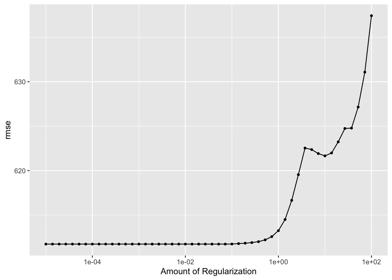

# Get RMSE from tuning results
rmse_values <- collect_metrics(LASSO_tune_results_CV) %>%
  filter(.metric == "rmse")
rmse_values

# A tibble: 50 × 7
     penalty .metric .estimator  mean     n std_err .config              
       <dbl> <chr>   <chr>      <dbl> <int>   <dbl> <chr>                
 1 0.00001   rmse    standard    612.    25    18.5 Preprocessor1_Model01
 2 0.0000139 rmse    standard    612.    25    18.5 Preprocessor1_Model02
 3 0.0000193 rmse    standard    612.    25    18.5 Preprocessor1_Model03
 4 0.0000268 rmse    standard    612.    25    18.5 Preprocessor1_Model04
 5 0.0000373 rmse    standard    612.    25    18.5 Preprocessor1_Model05
 6 0.0000518 rmse    standard    612.    25    18.5 Preprocessor1_Model06
 7 0.0000720 rmse    standard    612.    25    18.5 Preprocessor1_Model07
 8 0.0001    rmse    standard    612.    25    18.5 Preprocessor1_Model08
 9 0.000139  rmse    standard    612.    25    18.5 Preprocessor1_Model09
10 0.000193  rmse    standard    612.    25    18.5 Preprocessor1_Model10
# ℹ 40 more rows

# Save file
figure_file <- here("ml-models-exercise", "LASSO_tune_plot2.png")
ggsave(filename = figure_file, plot=autoplot(LASSO_tune_results_CV), bg="white")

Here, we can see that our lowest RMSE is around 611 and our highest is at 637. These are higher than our previous models, but we are now using cross-validation to avoid overfitting. CV is leading to a higher RMSE because it is using actual samples to train and test the data, creating a more generalizable model that is less likely to overfit. This model, even though it has a higher RMSE, is probably a better model since it is not overfitting.

Now let’s do the random forest model.

# Set seed for reproducibility
set.seed(rngseed)

# Create new recipe for random forest tuning model with CV
mavo_recipe_rf_tune_CV <- recipe(Y ~ ., data = mavo_ml)

#Define model specification using ranger
rf_spec_CV <-
  rand_forest(mode = "regression",
              mtry = tune(),
              min_n = tune(),
              trees = 300) %>% # number of trees
  set_engine("ranger", seed = rngseed)

# Create workflow for tuning
rf_tune_wf_CV <- workflow() %>%
  add_model(rf_spec_CV) %>%
  add_recipe(mavo_recipe_rf_tune_CV)

# Define parameter grids
param_grid2 <- grid_regular(
  mtry(range = c(1, 7)),
  min_n(range = c(1, 21)),
  levels = 7)

# Define the parameter mtry and create a grid for tuning, Used this website: https://dials.tidymodels.org/reference/mtry.html
#mtry_grid <- mtry(range = c(1, 7)) %>%
            # grid_regular(levels = 7)

# Define the parameter min_n and create a grid for tuning. Used this website: https://dials.tidymodels.org/reference/trees.html
#min_n_grid <- min_n(range = c(1, 21)) %>%
            # grid_regular(levels = 7)

# Combine grids
#param_grid <- expand_grid(mtry_grid, min_n_grid)

# Create CV samples
real_resamples2 <- vfold_cv(mavo_ml, v = 5, repeats = 5)

# Tune with control parameters
rf_tune_results_CV <- rf_tune_wf_CV %>% tune_grid(
  resamples = real_resamples2,
  grid = param_grid2,
  metrics = metric_set(rmse)
)

# Observe process
rf_tune_results_CV %>% autoplot()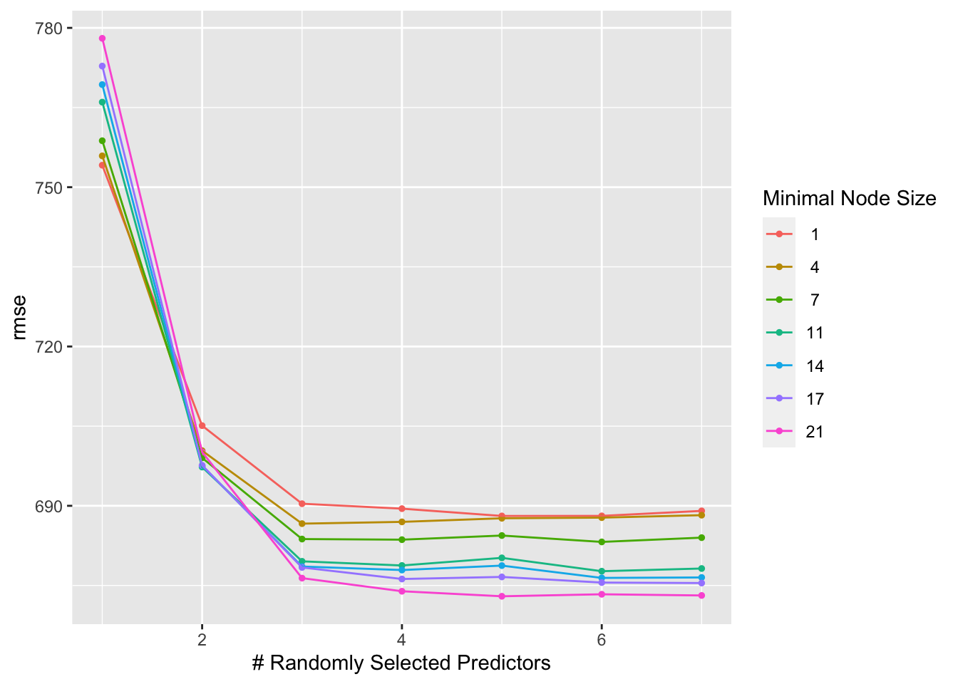

# Get RMSE from tuning results
rmse_values <- collect_metrics(rf_tune_results_CV) %>%
  filter(.metric == "rmse")
rmse_values

# A tibble: 49 × 8
    mtry min_n .metric .estimator  mean     n std_err .config              
   <int> <int> <chr>   <chr>      <dbl> <int>   <dbl> <chr>                
 1     1     1 rmse    standard    754.    25    26.1 Preprocessor1_Model01
 2     2     1 rmse    standard    705.    25    23.1 Preprocessor1_Model02
 3     3     1 rmse    standard    690.    25    22.2 Preprocessor1_Model03
 4     4     1 rmse    standard    689.    25    22.4 Preprocessor1_Model04
 5     5     1 rmse    standard    688.    25    22.6 Preprocessor1_Model05
 6     6     1 rmse    standard    688.    25    22.7 Preprocessor1_Model06
 7     7     1 rmse    standard    689.    25    23.1 Preprocessor1_Model07
 8     1     4 rmse    standard    756.    25    26.4 Preprocessor1_Model08
 9     2     4 rmse    standard    700.    25    23.3 Preprocessor1_Model09
10     3     4 rmse    standard    687.    25    22.2 Preprocessor1_Model10
# ℹ 39 more rows

# Define the file path
figure_file <- here("ml-models-exercise", "rf_tune_plot2.png")
ggsave(filename = figure_file, plot=autoplot(rf_tune_results_CV), bg="white")

The RMSE for the random forest model also increased, with the lowest at 673 and the highest at 769. Now, our CV-tuned LASSO has a lower RMSE than our random forest CV-tuned model. This makes sense given that one of the main disadvantages of tree models are that they have reduced performance compared to other models like LASSO. They are not good at high-performance prediction, which is what we were testing with the cross-validation. When using “fake” samples, the tree did better, but when faced with data it had not been trained on, the tree model fared worse than LASSO.